Activity 4.4.1. What’s in a Name.
Mathematics can be described as the study of patterns. For this reason, we often look for similar structure in both nature and mathematical systems. Mathematics can certainly be used to study patterns in the physical world, but we can also look for patterns within mathematics itself. Are there times when one mathematical system is, for all practical purposes, “identical” to another mathematical system and therefore governed by the same properties and relationships? If this is so, then one system can give us quite a bit of information about another system. In fact, if one system is easier to operate on, we can use it instead and then deduce information about the other system without having to do more difficult computations.
Recall that in Activity 4.3.6 we used the set of functions \(T=\left\{e, f, g, h, j, k\right\}\) under the operation of function composition where the functions are defined as follows:
\begin{equation*}
e\left(x\right)=x, f\left(x\right)=\frac{1}{x}, g\left(x\right)=\frac{x}{x-1}, h\left(x\right)=1-x,
j\left(x\right)=\frac{1}{1-x}, k\left(x\right)=\frac{x-1}{x}
\end{equation*}
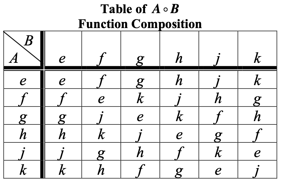
Further, recall that you found this set and operation to form a group and you constructed the Cayley (operation) table given below.
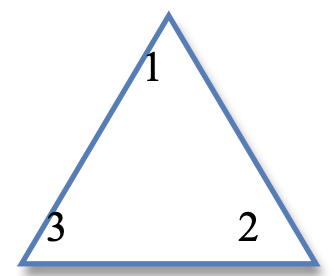
We will now consider a different set and operation. Take your equilateral triangle and mark the vertices 1, 2, and 3 on both faces (you will be flipping them over and will need to identify the same vertex from both faces of the triangle). Orient the triangle as shown in Figure 4.4.2.
(a)
Keeping the vertices labeled, how many different ways can you orient the triangle so that one side lies along the horizontal with the opposite vertex pointing upward? For example,
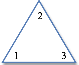
are different orientations.
(b)
Using the orientations you found in part (a) as the “basic” moves for the triangle, describe each orientation as a movement such as a flip or rotation from the original position given in Figure 4.4.2. For example, the movement described in part (a) could be considered a \(\frac{1}{3}\) or 120˚ counter-clockwise rotation or a \(\frac{2}{3}\) or 240˚ clockwise rotation.
(c)
In order to communicate with each other, we will decide on a common notation for moves of the triangle. Rotations will be clockwise. We will let \(r_0\) stand for no rotation, \(r_1\) denote a 120˚ rotation, and \(r_2\) represent a 240˚ rotation. For the flips, we have three axes about which we can flip the triangle (vertical and two diagonals). We will use \(v\text{,}\) \(d_1\text{,}\) and \(d_2\) to denote them as shown below.
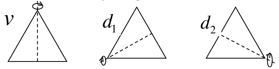
We will claim that these are the “basic” moves for the triangles so that it comes to rest back in the same “space” as it started. We will denote this set of moves as \(M=\left\{r_0, v, d_1, d_2, r_1, r_2\right\}\text{.}\) Explain how you know that these are the only “basic” moves. (think about how many ways you could re-label the triangle).
While we can use physical triangles to do these manipulations, we can also do it virtually by using matrix transformations. To help with performing the moves, we will use a set of matrices on the TI-Nspire CX CAS. These six matrices will take the original vertices and map them to their new locations. For your convenience, the matrices have been given names corresponding to our original names for the triangle moves as follows (see TI-Nspire document page 1.2).
\begin{equation*}
M=\left\{
\begin{array}
"r_0=\begin{bmatrix} 1 \amp 0\\ 0 \amp 1 \end{bmatrix}
\amp
r_1=\begin{bmatrix} -\frac{1}{2} \amp \frac{\sqrt{3}}{2}\\ -\frac{\sqrt{3}}{2} \amp -\frac{1}{2} \end{bmatrix}
\amp
r_2=\begin{bmatrix} -\frac{1}{2} \amp -\frac{\sqrt{3}}{2}\\ \frac{\sqrt{3}}{2} \amp -\frac{1}{2} \end{bmatrix}
\\
v=\begin{bmatrix} -1 \amp 0\\ 0 \amp 1 \end{bmatrix}
\amp
d_1=\begin{bmatrix} \frac{1}{2} \amp \frac{\sqrt{3}}{2}\\ \frac{\sqrt{3}}{2} \amp -\frac{1}{2} \end{bmatrix}
\amp
d_2=\begin{bmatrix} \frac{1}{2} \amp -\frac{\sqrt{3}}{2}\\ -\frac{\sqrt{3}}{2} \amp -\frac{1}{2} \end{bmatrix}
\end{array}
\right\}
\end{equation*}
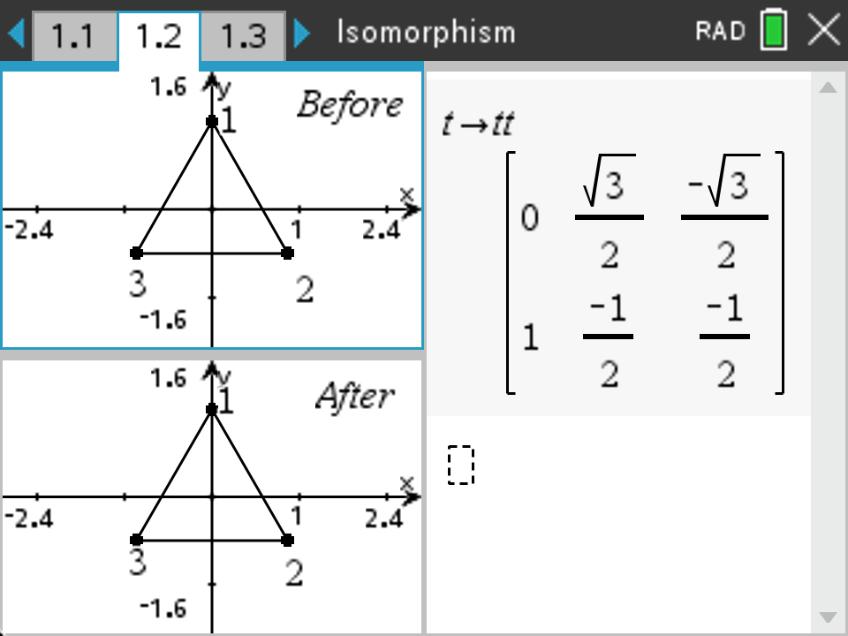
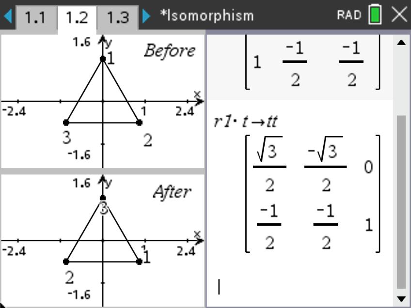
Here the triangle vertices are stored in a \(2 \times 3\) matrix, named \(t\) for “triangle”, where each column represents the \(x-\) and \(y-\)coordinates of vertices 1, 2, and 3 respectively as labeled on the triangle. The effect of matrix multiplication is that the vertices trade locations. For example, applying \(r_1\) to the triangle vertices matrix gives
\begin{equation*}
r_1 \cdot t=
\begin{bmatrix} -\frac{1}{2} \amp \frac{\sqrt{3}}{2}\\ -\frac{\sqrt{3}}{2} \amp -\frac{1}{2} \end{bmatrix}
\cdot \begin{bmatrix} 0 \amp \frac{\sqrt{3}}{2} \amp -\frac{\sqrt{3}}{2}\\ 1 \amp -\frac{1}{2} \amp -\frac{1}{2}
\end{bmatrix}=
\begin{bmatrix} \frac{\sqrt{3}}{2} \amp -\frac{\sqrt{3}}{2} \amp 0\\ -\frac{1}{2} \amp -\frac{1}{2} \amp 1
\end{bmatrix}
\end{equation*}
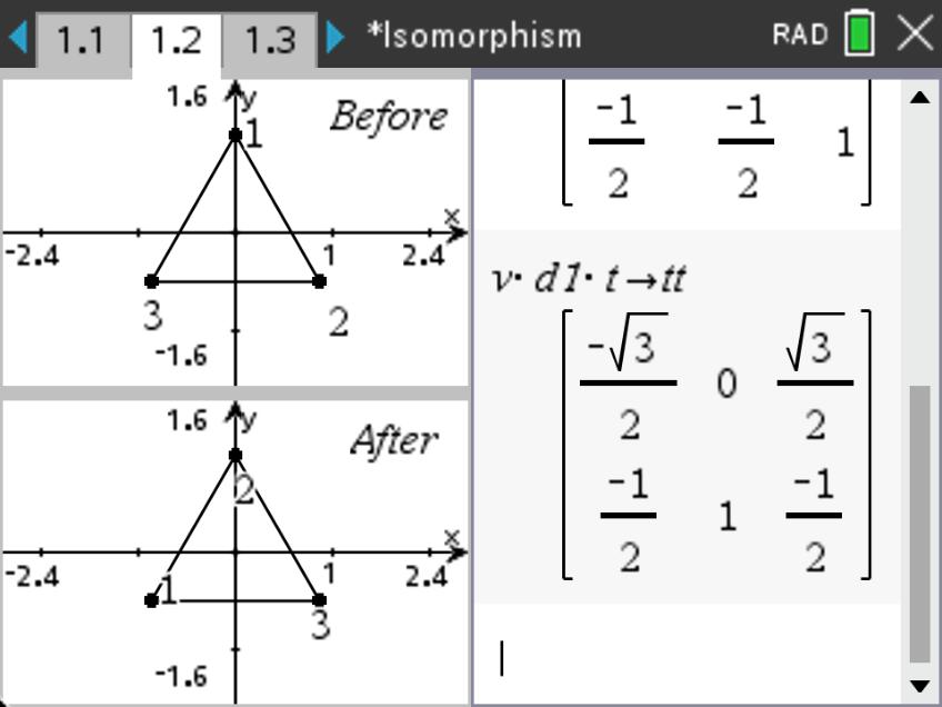
which is the same as rotating the triangle 120˚ clockwise. Notice that the coordinates of the vertices underwent the mappings \(\left(0,1\right) \mapsto \left(\frac{\sqrt{3}}{2}, -\frac{1}{2}\right)\text{,}\) \(\left(\frac{\sqrt{3}}{2}, -\frac{1}{2}\right) \mapsto \left(-\frac{\sqrt{3}}{2}, -\frac{1}{2}\right)\text{,}\) and \(\left(-\frac{\sqrt{3}}{2}, -\frac{1}{2}\right) \mapsto \left(0, 1 \right)\text{.}\) To see the changes from the original position displayed in the “Before” pane appear in the “After” pane of the screen, we perform the calculation and store the result in the matrix \(tt\) for “transformed triangle” (see screen images below). We can also perform multiple moves together. Consider applying the \(d_1\) flip followed by the \(v\) flip. This combination of moves yields an equivalent scenario as performing the \(r_2\) rotation (this has been filled in for you in the following operation table given in part (d)).
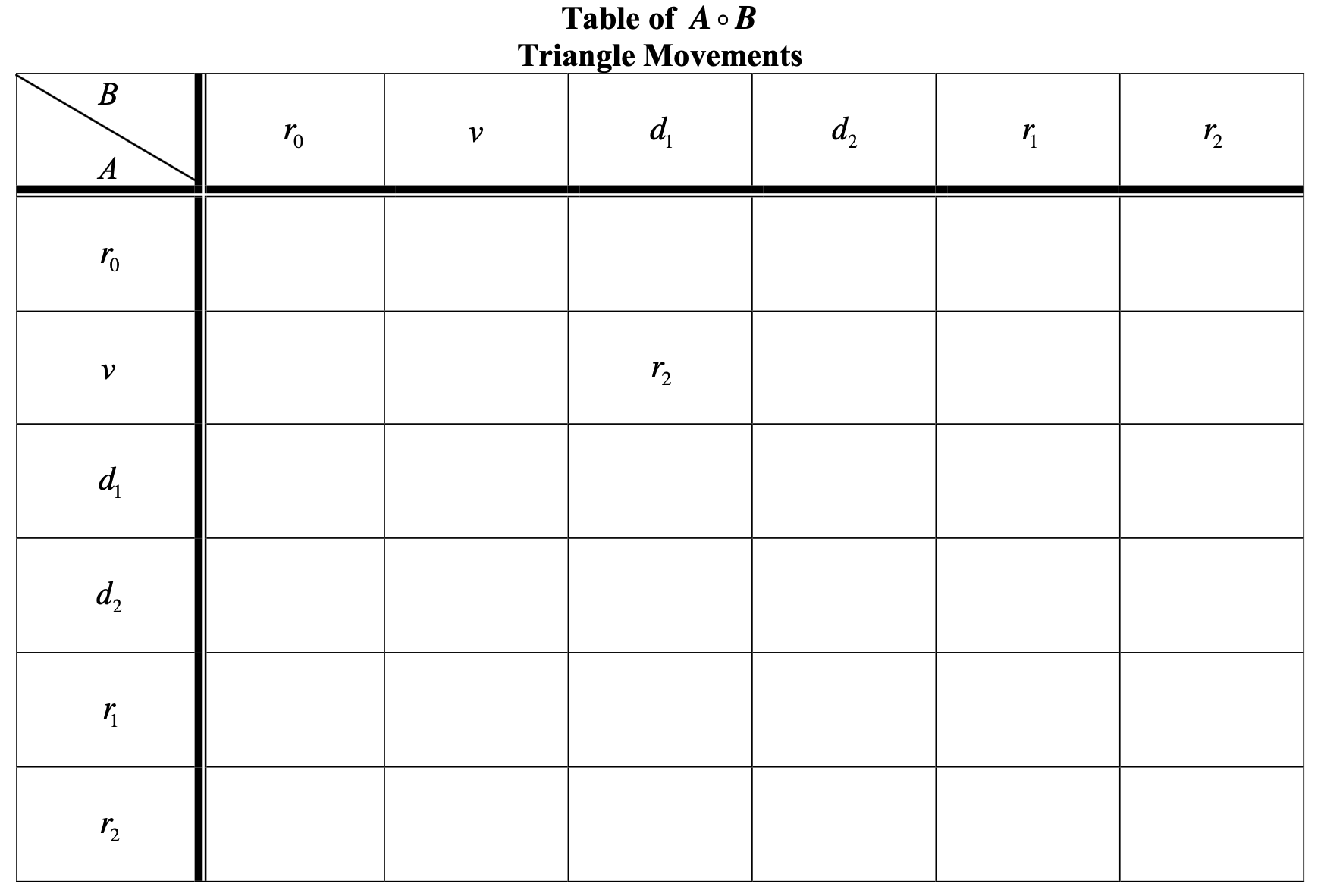
(d)
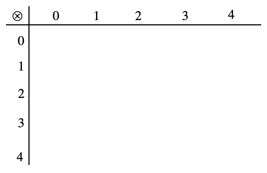
Build a table for the composition of the moves on the triangle of the form \(A \circ B\) where move \(B\) is performed first followed by move \(A\text{.}\) In the space below, record the result as shown.
(e)
In general, is the set of moves on the triangle closed under the operation of composition of moves? If not, what elements yield an element not in the original set of moves?
(f)
In general, do the elements of the set commute with each other? If not, do some of the elements commute with some of the other elements? Explain.
(g)
How might you check associativity? How many different permutations of these moves would you need to check to be certain of associativity? Devise a plan to check associativity. Your plan might include other groups from the class (divide and conquer is often very effective). Is there any pattern that you have noticed that might allow you to claim associativity without checking all possible combinations (consider your table of functions under composition from Figure 4.4.1)?
(h)
Is there a move from the set that acts like an identity element? If so, what is the move and explain how you know?
(i)
Does every element have an inverse? If so, list all elements and their inverses. If not, list any elements that do have an inverse along with their inverse element.
(j)
Again, recall that if a set along with an operation meets the four criteria of closure, associativity, an identity element, and all elements have inverses, then we call the set a group. Does this set of six moves on a triangle under the operation of composition of moves form a group?
(k)
Now consider the Cayley table you have just created. What similarities do you notice in relation to the earlier Cayley table of the group of six functions (see Figure 4.4.1)? What differences do you notice?
(l)
Given your observations about each set and operation, explain how you could use the table for function composition on \(T\) to answer questions about set \(M\) and its composition of movements on the triangle. (Think about ideas such as element orders and inverses).
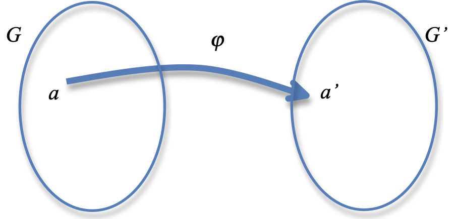
When looking at these two groups, you might have noticed similarities for the behavior among the elements of each group. We can think of these two groups as parallel universes where the relationships among the “people” of the two universes are the same within each world. We can therefore give a mapping between the worlds that tells who in one world corresponds to their similar person (doppleganger) in the other world. Let’s call this mapping \(\varphi\) where if the person, \(a\text{,}\) in the first world behaves like person, \(a'\text{,}\) in the other world, then \(\varphi\left(a\right)=a'\) (see the diagram below).
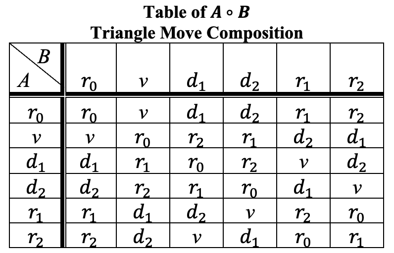
We can notice the similarity in behavior among the elements if we look at the Cayley tables side-by-side. Consider the Cayley table you just constructed shown next to the one that you created in Activity 4.3.6 shown below in Figure 4.4.3.
(m)
Give a mapping between sets \(T\) and \(M\) that describes how elements of \(T\) have similar behavior as elements in \(M\) only with a different operation. For example, if you thought that the function \(f\) in the group of functions behaved like the vertical flip in the group of triangle moves, you would write \(\varphi\left(f\right)=v\text{.}\) Describe what properties of the elements helped to decide what elements from \(T\) mapped to elements from \(M\text{?}\)(n)
In the earlier example, we thought of the set we were operating on as the set of “moves” on the triangle with the operation being composition of “moves”. What if we instead considered the set of elements to be the set of matrices given by
\begin{equation*}
S=\left\{
\begin{array}
"\begin{bmatrix} 1 \amp 0\\ 0 \amp 1 \end{bmatrix}
\amp
\begin{bmatrix} -\frac{1}{2} \amp \frac{\sqrt{3}}{2}\\ -\frac{\sqrt{3}}{2} \amp -\frac{1}{2} \end{bmatrix}
\amp
\begin{bmatrix} -\frac{1}{2} \amp -\frac{\sqrt{3}}{2}\\ \frac{\sqrt{3}}{2} \amp -\frac{1}{2} \end{bmatrix}
\\
\begin{bmatrix} -1 \amp 0\\ 0 \amp 1 \end{bmatrix}
\amp
\begin{bmatrix} \frac{1}{2} \amp \frac{\sqrt{3}}{2}\\ \frac{\sqrt{3}}{2} \amp -\frac{1}{2} \end{bmatrix}
\amp
\begin{bmatrix} \frac{1}{2} \amp -\frac{\sqrt{3}}{2}\\ -\frac{\sqrt{3}}{2} \amp -\frac{1}{2} \end{bmatrix}
\end{array}
\right\}
\end{equation*}
where the operation on the set is regular matrix multiplication. Explain why \(\left(S, \cdot \right)\) forms a group. How is this different than when we considered the group \(\left(M, \circ \right)\) where \(\circ\) refers to composition of “moves” on a triangle? How is it the same? How is it different than when we used \(\left(T, \circ \right)\) where \(\circ\) refers to composition of functions? How is it the same?
While we have looked at the movements on the triangle through the view of a physical triangle operated on by “moves” and as a set of matrices operated on by regular matrix multiplication used to actually perform the transformation of the physical triangle, we can also view it in another way. We could simply look at how the numbered vertices of the triangle are reassigned (or permuted). The ways in which the labels can be reassigned are called permutations and we can think about them as a mapping or function that assigns the old label of a vertex a new label from the same set of labels. Consider the following permutation of the labels:
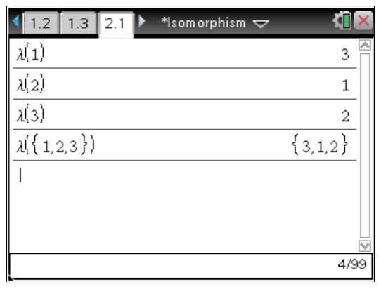
Here the labels for the vertices have undergone the following mappings where \(1\mapsto 3\text{,}\) \(2 \mapsto 1\text{,}\) and \(3\mapsto 2\text{,}\) meaning that 1 moved to what was 3’s location, 2 moved to what was 1’s location, and 3 moved to what was 2’s location. We can think of this as a function, \(\lambda\text{,}\) such that \(\lambda \left(1\right)=3\text{,}\) \(\lambda \left(2\right)=1\text{,}\) and \(\lambda \left(3\right)=2\) (see the first image in Figure 4.4.4). We could also think of performing the mapping in one fell swoop to the entire original set of labels, \(\left\{1,2,3\right\}\) yielding the output \(\left\{3,1,2\right\}\) by using braces “{}” (see the second image in Figure 4.4.4). In the early study of these permutations an array was used to convey the meaning of the mapping of labels to labels. In this case we can think of \(\lambda\) as \(\lambda =\left(\begin{matrix} 1 \amp 2 \amp 3 \\
\downarrow \amp \downarrow \amp \downarrow\\
3 \amp 1 \amp 2
\end{matrix}\right)\) where the mapping is viewed as a vertical assignment of labels. More simply we denote this as \(\lambda =\left(\begin{matrix} 1 \amp 2 \amp 3 \\
3 \amp 1 \amp 2
\end{matrix}\right)
\text{.}\)
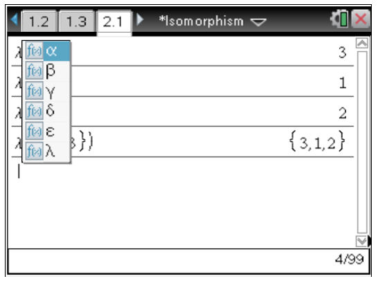
We will now consider the set of permutations (or functions), \(S_3\text{,}\) on the labels \(S=\left\{1,2,3\right\}\) as \(S_3=\left\{\alpha, \beta, \gamma, \delta, \epsilon, \lambda \right\}\text{.}\) To use these functions on your CAS, on page 2.1 of the Nspire document, press the
var key and select the given function name from the pop-up list (see the third image in Figure 4.4.4).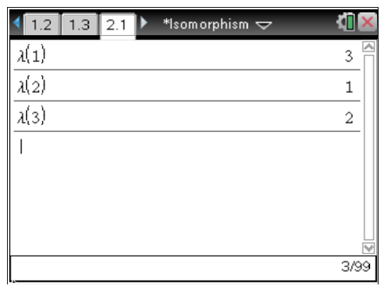
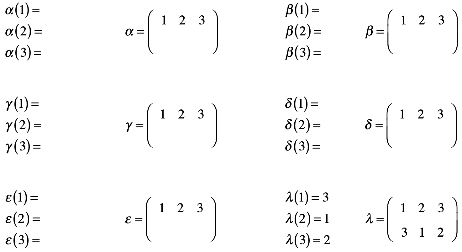
(o)
Using your CAS, fill in the following values using both regular function notation for individual elements of \(S\) as well as array notation for each function in \(S_3\text{.}\) Notice that the mapping for \(\lambda\) has been done for you as an example.
Since writing these permutation using two rows is time consuming, we have decided to write them using what is called cycle notation that only records what changes. For example since \(\lambda\) takes \(1\mapsto 3\text{,}\) \(3\mapsto 2\text{,}\) and \(2\mapsto 1\text{,}\) we use one row of labels to communicate this. Think of it as \(\lambda=\left(\underleftarrow{1\rightarrow 3 \rightarrow 2}\right)\) or more simply \(\lambda=\left(132\right)\text{.}\) If we consider a permutation that leaves a label unchanged, we simply do not write it. For example, suppose we have \(\left(\begin{matrix} 1 \amp 2 \amp 3 \\
3 \amp 2 \amp 1
\end{matrix}\right)\) where 2 stays fixed and 1 and 3 swap positions. Here we would write this as \(\left(\begin{matrix} 1 \amp 2 \amp 3 \\
3 \amp 2 \amp 1
\end{matrix}\right)=\left(13\right)\left(2\right)\) or more simply \(\left(13\right)\) leaving out any fixed labels.
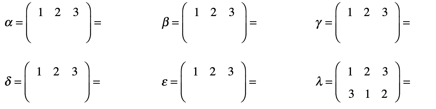
(p)
Now take the array notation you found in the last question and write it in cycle notation.
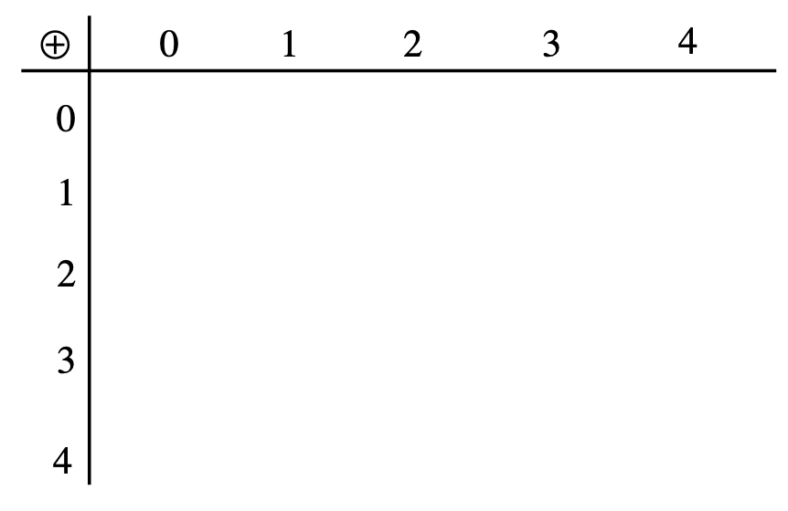
(q)
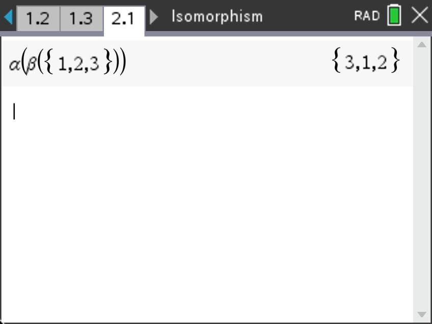
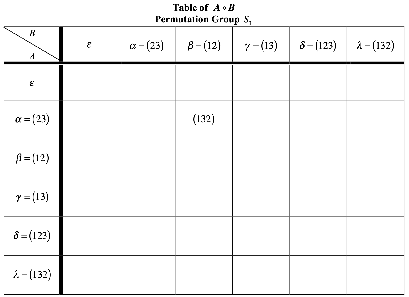
Now using the elements of the permutation group, \(S_3\text{,}\) expressed in cycle notation, fill in the Cayley table in Figure 4.4.5. You can use the CAS to help with these. For example, to perform \(\alpha \circ \beta\) as shown in the table, you can simple enter \(\alpha \left(\beta \left(\left\{1,2,3\right\}\right)\right)\) on the CAS to get \(\left\{3,1,2\right\}\) (see image below) meaning \(\left(\begin{matrix} 1 \amp 2 \amp 3 \\
3 \amp 1 \amp 2
\end{matrix}\right)=\left(132\right)
\text{.}\)
(r)
In looking at the Cayley table for permutations you have just constructed, describe what you notice about the structure of the table. Have you seen this group before? Explain.
At this point we have seen how different sets of elements and different operations display behavior that is “the same” in some sense. As Poincaré stated, “Mathematicians do not study objects, but relations among objects; they are indifferent to the replacement of objects by others as long as relations do not change. Matter is not important, only form interests them.” Basically what he meant is that mathematicians are really more concerned with an overall structure (or behavior), not necessarily the particular set or operation used. So how do we define what you observed in the earlier questions—namely that the sets and operations used, \(\left(T, \circ\right)\text{,}\) \(\left(M, \circ\right)\text{,}\) \(\left(S, \cdot\right)\text{,}\) and \(\left(S, \circ\right)\) are basically the same from a behavioral standpoint? There are really three main properties that have to be met to define what we mean by “same behavior”. Consider the mapping we defined earlier between different “worlds” where, for example, \(\varphi\left(f\right)=v\text{.}\)
(s)
What two properties of functions must be true about the function \(\varphi\) to say, “every element in one world is mapped to exactly one element on the other world and no element in any world goes unmapped”? Explain your thinking.
(t)
Suppose you take two functions in the group \(\left(T, \circ\right)\) and combine them before mapping them to the group \(\left(M, \circ\right)\text{.}\) Here you might have \(\varphi\left(f\circ g\right)=\varphi\left(k\right)=r_2\text{.}\) Explain what you get if you do the mapping of each element into the group \(\left(M, \circ\right)\) first before you compose the resulting elements under the operation in \(\left(M, \circ\right)\text{.}\) In other words, what are \(\varphi\left(f\right)\) and \(\varphi\left(g\right)\) and then what do you get when you perform \(\varphi\left(f\right) \circ \varphi\left(g\right)\text{?}\) In general, what can you say will always be true for the mapping of any two elements \(\varphi\left(ab\right)\) if \(\varphi\left(a\right)\) and \(\varphi\left(b\right)\) are to “behave” like \(a\) and \(b\) do in their respective group. We call this operation preserving under the mapping.
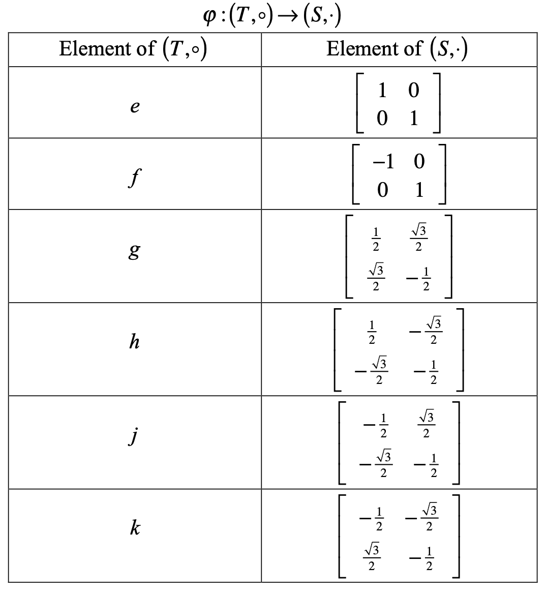
(u)
Now suppose \(\varphi : \left(T,\circ\right) \rightarrow \left(S, \cdot\right)\) defined by the table in Figure 4.4.6. Without actually finding the composition, \(g \circ j\text{,}\) what will you get if you perform \(\varphi\left(g \circ j\right)\text{?}\) Now perform \(g \circ j\) first and see if it maps to what you expected. Describe what you notice.
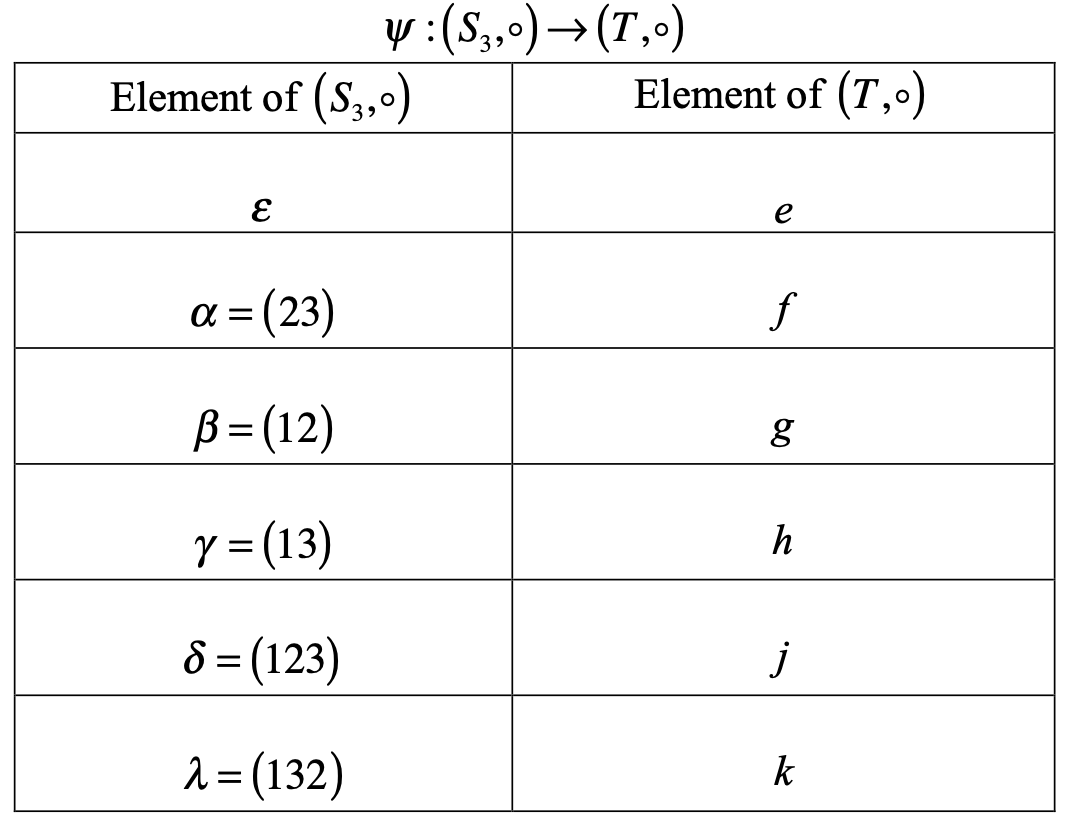
(v)
Consider the mapping, call it \(\psi\text{,}\) between \(S_3\) and \(T\text{,}\) \(\psi : \left(S_3,\circ\right) \rightarrow \left(T, \circ \right)\) given in Figure 4.4.7, and without actually finding the composition \(\left(23\right) \circ \left(12\right)\) first, find \(\psi\left(\left(23\right) \circ \left(12\right)\right)\) and record what you would expect to get [Feel free to use the Cayley table given for \(T\) from Figure 4.4.1]. Now perform \(\left(23\right) \circ \left(12\right)\) and see if it maps to what you expected. Describe what you notice.