Section4.3Inverses, Undoing, and the Role of Structure
As we examine the nature of algebra, we might begin by asking the question, "What is it good for?". Think back to your early experiences with algebra in middle or high school. What would you say was its purpose? You will likely recall spending a great deal of time solving equations. In fact, much of the processes and procedures that you spent substantial time mastering were in pursuit of solutions to equations. But how and why do these processes and procedures work? To answer this question, we need to examine the "structure" that is algebra.
Activity4.3.1.
Suppose you wanted to solve the equation, \(x+5=8\text{.}\) What processes would you use to solve it? For each of the following stages of the solution process, provide a mathematical property that was used to transform the equation to its new form.
Distributive Property of Multiplication over Addition
Zero Property of Multiplication
(d)
\begin{equation*}
x+0=3
\end{equation*}
\begin{equation*}
x=3
\end{equation*}
Hint.
Choose from:
Associative Property of Addition
Additive Identity
Additive Inverse
Addition Property of Equality
Distributive Property of Multiplication over Addition
Zero Property of Multiplication
(e)
Could you use your process if the only set of numbers allowed was the set of integers, \(\mathbb{Z}\text{?}\)
(f)
Could you use your process if the only set of numbers allowed was the set of real numbers, \(\mathbb{R}\text{?}\)
In Activity 4.3.1, you identified mathematical properties at each stage of the solution process. But is there truly a "structure" to this process? If so, can this structure be abstracted and can it be used in other cases for solving equations? Consider the following activity.
Activity4.3.2.
Suppose you wanted to solve the equation, \(7x=28\text{.}\) What processes would you use to solve it? For each of the following stages of the solution process, provide a mathematical property that was used to transform the equation to its new form.
Distributive Property of Multiplication over Addition
Zero Property of Multiplication
(d)
\begin{equation*}
1 \cdot x=4
\end{equation*}
\begin{equation*}
x=4
\end{equation*}
Hint.
Choose from:
Associative Property of Multiplication
Multiplicative Identity
Multiplicative Inverse
Multiplicative Property of Equality
Distributive Property of Multiplication over Addition
Zero Property of Multiplication
(e)
Could you use your process if the only set of numbers allowed was the set of integers, \(\mathbb{Z}\text{?}\)
(f)
Could you use your process if the only set of numbers allowed was the set of real numbers, \(\mathbb{R}\text{?}\)
(g)
Looking at the mathematical properties you used in Activity 4.3.1, describe any pattern you see with respect to parts (a)-(d) of this activity.
(h)
In Activity 4.3.1, you used addition as the operation within the equation. In this activity, you used multiplication. Suppose you have an equation that uses only one operation, summarize the basic properties that are essential in order to solve an equation.
The properties that you just noticed in trying to solve the equations in Activity 4.3.1 and Activity 4.3.2 are the basic and essential properties that are required to solve an equation that uses only one binary operation. For this reason, it should come as no surprise that the most basic structure we define in algebra is composed of these properties. We call a structure that has these four properties a group and we will spend some time looking at the behavior of groups and examine how these structures are actually taught in the secondary algebra curriculum.
Definition4.3.1.
A group is a set, \(G\) along with a binary operation, \(*\text{,}\) such that if \(a,b,c \in G\) the following properties hold.
Closure : If \(a,b \in G\text{,}\) then \(a*b \in G\text{.}\)
Associativity : If \(a,b,c \in G\text{,}\) then \(a*\left(b*c\right)=\left(a*b\right)*c\text{.}\)
Identity : There exists an element, \(e \in G\text{,}\) (called the identity) such that \(e*a=a*e=a\) for all \(a \in G\text{.}\)
Inverses : For all \(a \in G\text{,}\) there exists an inverse element, denoted \(a^{-1}\text{,}\) such that \(a*a^{-1}=a^{-1}*a=e\text{.}\)
Think back to when you first decided to become a secondary mathematics teacher. Now recall your reaction when you learned how much mathematics you had to take to complete the degree. Often preservice mathematics teachers contemplate entering the profession thinking, “Well, I’ve been through high school math so becoming a math teacher shouldn’t be too difficult. After all, it only involves learning how to present the mathematics I already know.”
When listening to university students talking in the hallways, it is not uncommon to hear comments such as, “Why do I have to take Abstract Algebra, I’m never going to teach this stuff to high school students?” Lurking in the background is the assumption that they have a deep knowledge of the mathematics that makes up the secondary curriculum. Unfortunately, most high school students’ perception of algebra involves symbol manipulations and memorized formulae and algorithms. In order to address the underlying structure of mathematics, we will examine a basic skill that is taught in the secondary schools from an advanced standpoint.
Subsection4.3.1The Concept of Inverse: Setting the Stage
In order to begin a fruitful discussion of mathematical concepts and their relationship to teaching and learning, it is helpful to first examine our own understanding of the concepts in question. In this particular section, we will investigate the concept of inverse function. From a constructivist perspective, no two people have exactly the same conceptual understanding of inverse function. While there may be some common definitions and representations used for describing this idea, not all people have the same mental constructs and images that emerge when the term “inverse function” is mentioned. The way in which other mathematical ideas are connected to this concept may also be quite different depending on the person you ask. Here you will be asked to give some preliminary responses to questions and to build a concept map showing your linkages among mathematical ideas.
Activity4.3.3.
We begin by reflecting on our own understanding of inverse. In your own words, respond to the following questions with respect to your current conception of "inverse function".
(a)
In relation to the concept of function, describe what the term “inverse function” means?
(b)
Describe how you came to understand the concept of inverse function.
(c)
Imagine yourself in your first teaching position where you have to teach students about inverse functions, how would you teach it? How is it connected to other mathematics they have learned (i.e. what would Pirie & Kieren give as the primitive knowing for expanding the concept of inverse function)?
One of the ways in which we advance our thinking is through reflection. In Activity 4.3.3, you began by describing your understanding of a concept. At this point it is important to reflect on your responses and try to articulate your understanding in greater detail. To accomplish this task, we will use a concept map to pull your mental constructs together and prompt you to reflect on your own understanding.
Activity4.3.4.
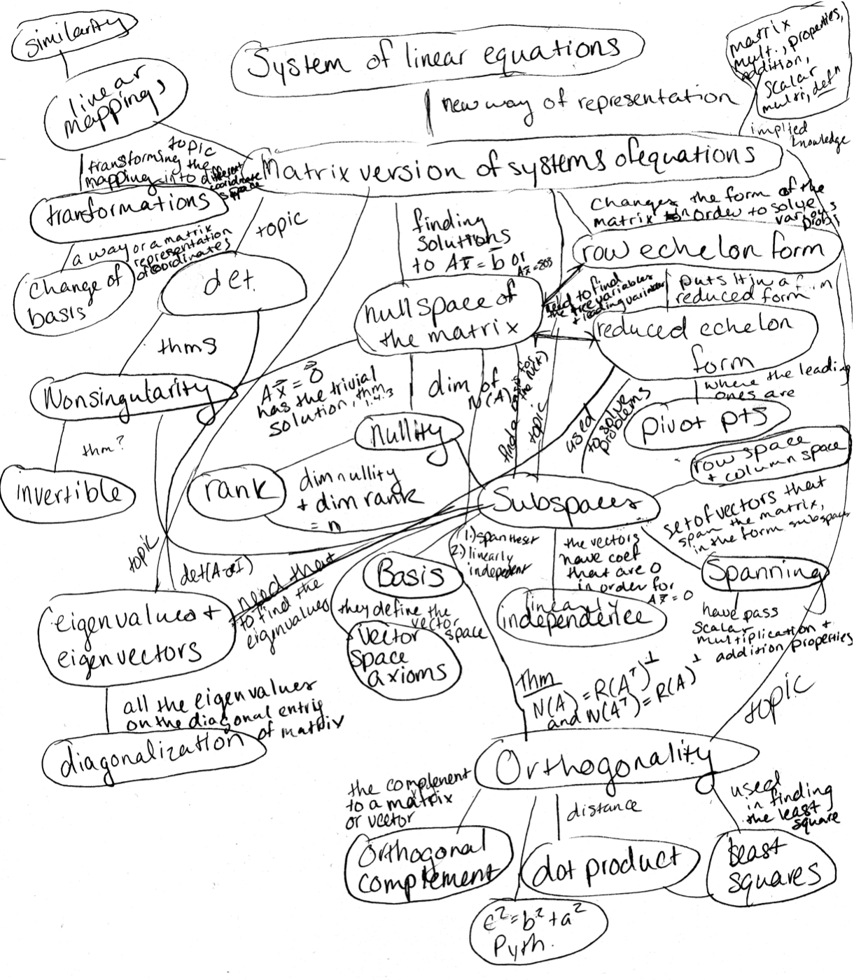
A concept map is like a flow chart; however, there is not necessarily a linear flow of ideas. Instead, it is often the case that the concept map resembles more of a web with concepts connected in a variety of ways. Figure 4.3.2 gives a sample of a concept map constructed by a student showing relationships within concepts from a Linear Algebra course. The main aspects of the maps are the concept (usually encased in a bubble) and segments or directed line segments showing how the concepts are connected. In some cases, the connections are bidirectional; in others they may only go one way. These connections usually have words or symbols written along them to explain how the person views the connection between the two concepts.
Figure4.3.2.Sample Concept Map for Linear Algebra
(a)
Using all related concepts you can think of, create a concept map for the concept of inverse function.
(b)
Share your concept map with other members of your group. On your whiteboards, summarize commonalities in your group members’ maps. Summarize some of the ways in which group members gave a unique connection on their maps.
Now that you have started to reflect on the concept of inverse function, consider the following classroom exchange as a teacher (Tim) interacts with his students. Following the vignette, you will be asked to respond to questions surrounding the discussion.
Activity4.3.5.Inverse Functions: The Case of Tim.
Tim is a beginning teacher in his second year. Today, he is teaching the concept of inverse function. To find an inverse function, the text that Tim is using begins by having the students swap the variables of \(x\) and \(y\) and then solve for \(y\text{.}\) He is fairly confident that he can teach his students how to use this procedure to find inverse functions, but also noted that the book has students check to see if the inverse function works by composing the two functions to see if the composition results in “x”. Tim also noticed that the book covers function composition in the section before inverse function and assumes this is so that students can understand how to check their answers once they have found the inverse function. Since he wants to be sure the students are ready, he begins class by discussing the previous day’s lesson on function composition.
Tim : OK, let’s make sure we understand what we did yesterday since we are going to use it today. What is composition of functions?
Jen : Isn’t it just sticking one thing into another?
Tim : Yes, it is. Can anyone show us how to do it? [Lori raises her hand]. Lori, go to the board. Can anyone give us two functions? [Ken raises his hand]. Ken, whatcha got?
Ken : How about \(f\left(x\right)=3x-1\) and \(g\left(x\right)=x^2+x\text{?}\)
Tim : Great. Now Lori, show us what to do.
Lori : OK, I guess it depends on what order you want.
Tim : Let’s do \(f\left(g\left(x\right)\right)\text{.}\)
Lori : So we just take \(x^2+x\) and stick it in for \(x\) in \(3x-1\text{.}\) That gives us \(3\left(x^2+x\right)-1\text{.}\) Now we can just distribute it out and that gives us \(3x^2+3x-1\text{.}\)
Tim : Super! Is everyone OK with that? [The class is quiet]. Good, let’s move on to today’s stuff. Thanks, Lori. [Lori sits down].
Tim : Today we’re going to look at inverses when it comes to functions. Has anyone ever heard the word “inverse” before? [Several hands go up]. Yeah, Mia.
Mia : Wouldn’t that just be like the flip of a function?
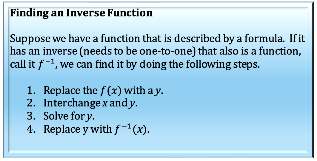
Tim : [Smiles]. No, that’s a common mistake. This is completely different when it comes to functions. Let’s look at the book’s way of finding inverse functions. In pairs, take a couple of minutes to read the procedure on page 213 (see Figure 4.3.3).
Figure4.3.3.Excerpt from Tim’s Text
[Students are given 5 minutes to read and discuss the procedure as Tim circulates observing their discussions. Tim notices that in the pair of Mike and Sam, Mike seems to be doing most of the explaining and so plans to call on Mike.]
Tim : Mike, in your own words explain how to find inverse functions.
Mike : Well, first you just switch the \(x\) and \(y\)s. Then you just solve for \(y\) so that \(y\) is on one side of the equation and the other side just has \(x\)s.
Tim : Very good. Let’s do one together. Let’s start with lines. How about the function we used earlier, \(y=3x-1\text{.}\) Tell me what to do. Yeah, Joan, get us started.
Joan : First write it as \(x=3y-1\text{.}\)
Tim : Now what? Someone else [Hiro raises his hand]. Hiro go ahead.
Hiro : Just add 1 to both sides to get \(x+1=3y\text{.}\) The only thing we have to do now is divide by 3 so we get \(y\) all by itself. That gives us \(y=\frac{x+1}{3}\text{.}\)
Tim : Excellent. Does everyone see how it’s done? [Kat raises her hand]. Yeah, Kat.
Kat : How do we know it’s the inverse function?
Tim : I’m glad you asked that, Kat. That’s our next part of the lesson. To see if it worked, we just think of these as functions and compose them like we did yesterday. If we get “x”, then they are inverses. Let’s try it. OK, let’s make \(f\left(x\right)=3x-1\) like we did before and now make \(g\left(x\right)=\frac{x+1}{3}\text{.}\) Sue, come to the board and work out this composition.
Sue : [Sue goes to the board and begins writing.] OK, we have \(f\left(g\left(x\right)\right)\text{.}\) That gives \(3\left(\frac{x+1}{3}\right)-1\text{.}\) We can cancel the 3s and that leaves just \(x+1\) and \(-1\text{.}\) The 1 and -1 cancel and we get \(x\text{.}\)
Tim : Great. Do you see, Kat? Since we got \(x\) that means they’re inverses.
Kat : I’m still not sure how you know they’re inverses?
Tim : Well, we got \(x\text{.}\) If you compose a function and its inverse you get \(x\text{.}\) Let’s do a few more and that might help with remembering it.
Kat : But why do we get \(x\text{?}\) Why don’t we get 1?
Tim : That’s just the definition of what it means to be an inverse function. Just follow these steps and you’ll be OK.
[Kat gives a frustrated look and pulls out another sheet of paper.]
(a)
Describe the central issues involved in the classroom exchange.
(b)
At one point a student, Mia, offers up an explanation of what is meant by an inverse function. In response to this, Tim (the teacher) says, “No, that’s a common mistake. This is completely different when it comes to functions. Let’s look at the book’s way of finding inverse functions. In pairs, take a couple of minutes to read the procedure on page 213.”. Discuss your thoughts on Tim’s response.
Subsection4.3.2Inverse and Algebraic Structure
Now that we have started to reflect on our own experiences with inverses, we need to spend a little time exploring inverses beyond the elementary operations of addition and multiplication. While these early experiences ground us in similar patterns of behavior of sets of numbers with each operation, we need to branch out to other sets of object and operations in order to begin to abstract these behaviors and not worry about the context in which they live. After all, Poincaré expressed this so well.
Mathematicians do not study objects, but relations among objects; they are indifferent to the replacement of objects by others as long as relations do not change. Matter is not important, only form interests them. — Henri Poincaré.
As we saw in Tim’s class from Activity 4.3.5, Kat was frustrated by the response she received from Tim when her expectation of obtaining a 1 when composing a function and its inverse did not occur. In addition to this, Mia tried to explain her understanding of inverse by stating, "Wouldn’t that just be like the flip of a function?". To which Tim smiled and responded, "No, that’s a common mistake. This is completely different when it comes to functions." Instead of taking these two responses and noticing the commonality (both students seemed to be thinking of multiplication as the operation), Tim shut them down as if what they are about to learn with respect to inverse functions is a new concept. Pirie & Kieren would see the students’ responses as an opportunity to fold back to more familiar sets and operations where the students have comfort and build toward abstraction by prompting the learner to explore the underlying structure inherent in the behavior common to addition, multiplication, and function composition. To help us frame our discussion, let’s take a little mathematical detour and explore the same structure we noticed before we defined a group. Only this time, we will use sets of functions and our operation will be function composition, \(\circ\text{.}\)
Activity4.3.6.Form and Function.
This activity explores basic concepts of algebra including properties of algebraic structure. In high school, the primary operations used in algebra were multiplication and addition. Are these the only types of operations that can be used? We will explore this question and look for patterns that are common across algebra.
Recall that in your experiences in elementary school, you first learned to operate on the set of integers, \(\left\{\ldots, -3, -2, -1, 0, 1, 2, 3, \ldots \right\}\text{,}\) using a simple operation, addition. When this set was combined with the operation of addition, certain properties held. Some of these properties included: closure, associativity, the existence of an identity element, and inverses.
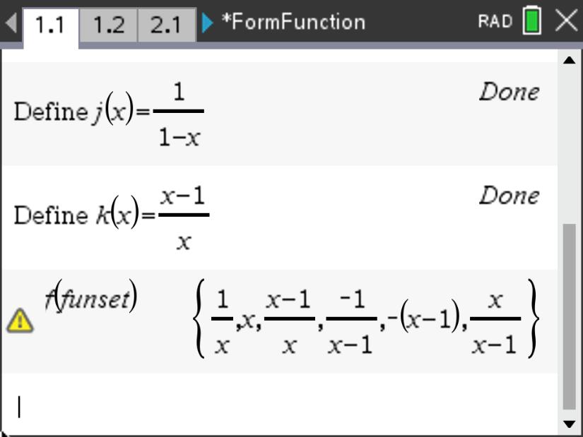
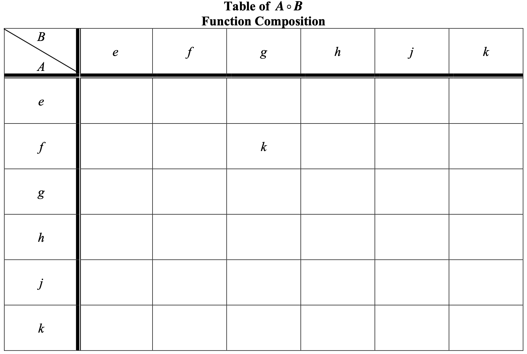
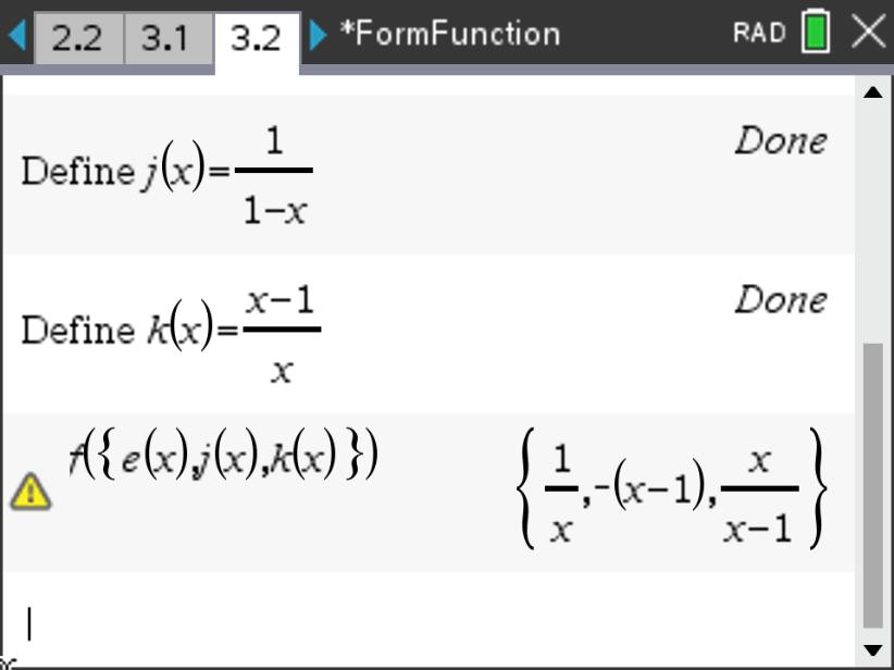
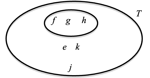
Consider the set of functions, \(T=\left\{e, f, g, h, j, k\right\}\text{,}\) where the functions are defined as follows:
Mathematics can be described as the study of patterns. For this reason, we often look for similar structure in both nature and mathematical systems. Mathematics can certainly be used to study patterns in the physical world, but we can also look for patterns within mathematics itself. Are there times when one mathematical system is, for all practical purposes, “identical” to another mathematical system and therefore governed by the same properties and relationships? If this is so, then one system can give us quite a bit of information about another system. In fact, if one system is easier to operate on, we can use it instead and then deduce information about the other system without having to do more difficult computations.
In this activity, we will explore what properties exist when pairing the set \(T\) above with the operation of composition of functions, \(\left(T,\circ \right)\text{.}\) As you explore this set, try to keep your eyes open for patterns in the relationships among functions. Some properties you may want to check might include: closure, associativity, identity, inverses, and commutativity. For example, consider your experience with basic arithmetic. For addition on the set of integers, the set is closed since adding two integers always results in another integer. The number 0 acts as an identity (i.e. \(a+0=0+a=a\text{,}\) leaving other elements unchanged) and 5 and -5 are inverses of each other (i.e. \(5+^{-}5=0\text{,}\) where combining them yields 0, the identity). This type of structure is very important for deducing mathematical truths within a mathematical system.
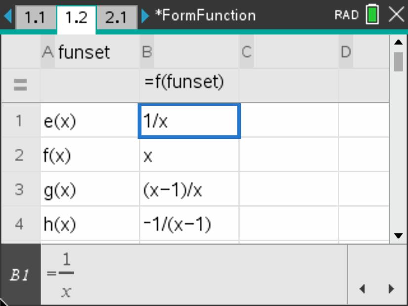
To begin, we define the functions above on your computer algebra system. This has already been done for you on page 1.1 of the TI-Nspire CAS document. Once the functions are defined, build an operation table (called a Cayley table) for the composition of functions of the form \(A \circ B\) in the space below by simply entering compositions such as \(f\left(g\left(x\right)\right)=\frac{x-1}{x}=k\left(x\right)\) and recording the result in the table as shown. This can be done more efficiently by first entering the functions in a spreadsheet (see page 1.2 of the FormFunction.tns file) and naming the entire set of functions “funset” and then performing compositions on the entire set all at once either on the Calculator page (or using the GeoGebra applet below in Figure 4.3.5) or in the Lists & Spreadsheets page (see Figure 4.3.4). If you use the spreadsheet, note that the columns in the spreadsheet correspond to rows in the table you are filling in due to the way the same operation is performed for an entire column in the spreadsheet. This syntax is similar to Microsoft Excel [i.e. by typing \(\mathbf{=f(funset)}\)].
Figure4.3.4.Composing Functions on the the Calculator and Lists & Spreadsheets apps
Figure4.3.5.Composition of Table Rows
(a)
In general, is the set \(T\)closed under the operation of composition of functions? In other words, when performing the operation on any two elements of the set, do you always get a result that is also an element of the set? If not, what elements yield an element not in \(T\text{?}\)
(b)
Recall that the associative property states that for any three elements under the operation, say \(*\text{,}\)\(a*\left(b*c\right)=\left(a*b\right)*c\text{.}\) How might you check associativity? How many different permutations of these functions would you need to check to be certain of associativity? Devise a plan to check associativity. Your plan might include other groups from the class (divide and conquer is often very effective).
(c)
Is there a function from the set that acts like an identity element? If so, what is the function?
(d)
Does every element have an inverse? If so, list all elements and their inverses. If not, list all elements that do have an inverse along with their inverse element.
(e)
Recall if a set along with an operation meets the four criteria of closure, associativity, an identity element, and all elements have inverses, then we call the set a group. Does this set of six functions under the operation of function composition form a group?
(f)
In general, do the elements of the set commute with each other? In other words, do you always get the same result when combining any two given elements in either order (commutativity)? If all of the elements of a group commute with each other, then the group is called abelian. If a group is abelian, what kind of symmetry would you see in its Cayley table?
(g)
If the group is not abelian, for each element of \(T\text{,}\) find all elements of \(T\) that do commute with it. In other words, find all elements of \(T\) that commute with \(e\text{,}\) then all elements of \(T\) that commute with \(f\text{,}\) then all elements of \(T\) that commute with \(g\text{,}\) …etc. Here you might want to use the Cayley table you created earlier along with your answer regarding the symmetry of the table for commutativity from part (f). We call each of these sets the centralizer of the element, denoted \(C\left(e\right)\text{,}\)\(C\left(f\right)\text{,}\)\(C\left(g\right), \ldots\text{.}\)
(h)
Now list all of the elements that the sets you found in part (g) have in common. In other words, find \(C\left(e\right) \cap C\left(f\right) \cap C\left(g\right) \cap C\left(h\right) \cap
C\left(j\right) \cap C\left(k\right)=\bigcap\limits_{a \in T} C\left(a\right)\text{.}\) Since each of these elements must commute with each and every element of \(T\) in order to be in the intersection, we call this special set of elements that commute with each other the center of\(T\) and denote it by \(Z\left(T\right)\text{.}\)
If a group would be abelian, what elements would be in its center?
(i)
On the Calculator page (page 2.1) of your CAS, if \(k\left(x\right)=\frac{x-1}{x}\text{,}\) find \(k^5\) if it is defined by \(k^n=\underbrace{k\circ k\circ k\circ \cdots \circ k}_\text{n times}\text{.}\) Note that a “power” here is not the usual “repeated multiplication”, but instead repeated composition of functions.
(j)
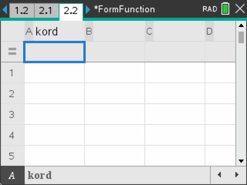
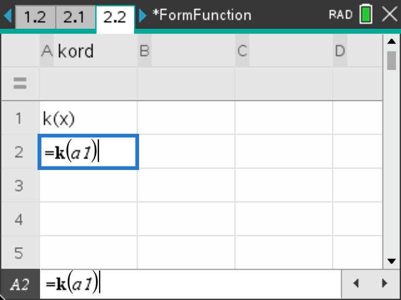
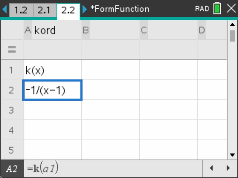
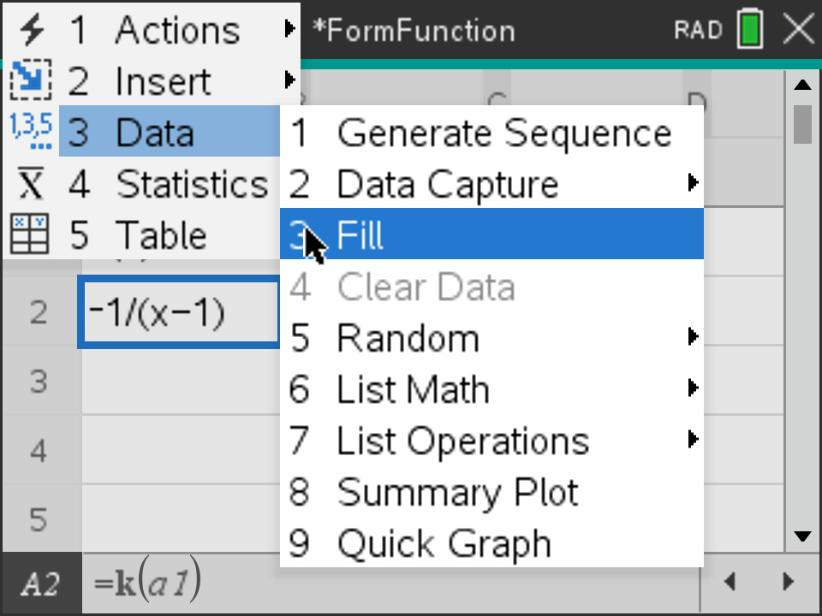
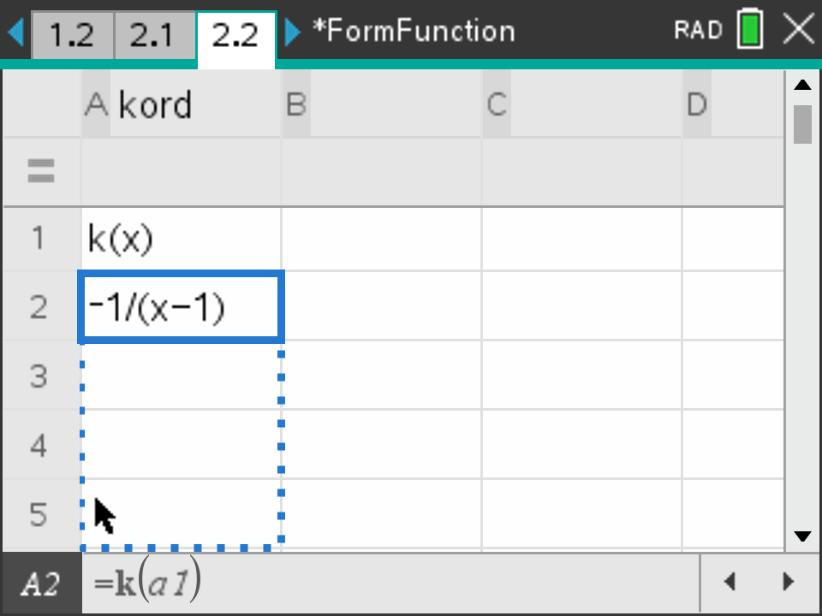
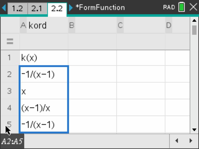
On page 2.2, use your algebraic spreadsheet to generate a sequence of \(k, k^2, k^3, \ldots, k^{10}\text{.}\) To do this, you can use the \(\mathbf{Fill Down}\) feature of the spreadsheet by first entering \(k\left(x\right)\) in the cell \(\mathbf{a1}\) and then in cell \(\mathbf{a2}\) entering \(=k\left(a1\right)\text{.}\) Then select cell \(\mathbf{a2}\) and choose menu\(\mathbf{3:Data}\) followed by \(\mathbf{3:Fill}\text{.}\) Using the down arrow key, move down in the spreadsheet about 8 cells or so and press enter· (See screens below for setting up the recursive composition). For what powers of \(k\) do you get \(k^n=e\text{?}\) Note that we labeled the column “kord” because this iteration will help us find what is called the order of the element \(k\text{.}\)
(k)
Using your algebraic spreadsheet to make a column for each function, repeat part (j) for the other functions in \(T=\left\{e,f,g,h,j,k\right\}\text{.}\) Label the columns “ford”, “gord”, “hord”, …etc. List the elements in each set produced. For example, in using the element \(k\text{,}\) you should get \(kord=\left\{k,j,e\right\}\text{.}\) You should notice that these elements just keep repeating and so the set is just limited to these three elements (note that when listing elements, we do not care about the order in which the elements are listed since they are just a set). Mathematically here we use the notation \(\langle k \rangle\) to mean the subgroup generated by\(k\) (i.e. repeatedly iterating \(k\) with itself \(\langle k \rangle=\left\{k, k^2, k^3, \ldots\right\}\)). In this case, \(\langle k \rangle\) is finite with order 3 since it begins to repeat. What can you say about the sizes of these subsets? Here the "size" or number of elements in the subgroup is called the order of the subgroup. State any patterns you notice.
\(\langle e \rangle=eord=\)
\(\langle f \rangle=ford=\)
\(\langle g \rangle=gord=\)
\(\langle h \rangle=hord=\)
\(\langle j \rangle=jord=\)
\(\langle k \rangle=kord=\)
(l)
List the smallest positive “power” for each element of \(T\) that yields, \(e\) [this is called the order of the element, denoted \(\lvert a \rvert\text{.}\) You can also think of this as the number of elements in the subsets produced in part (k)]. State any relationship you see between these powers and the number of elements in set, \(T\text{.}\)
\(\lvert e \rvert=\)
\(\lvert f \rvert=\)
\(\lvert g \rvert=\)
\(\lvert h \rvert=\)
\(\lvert j \rvert=\)
\(\lvert k \rvert=\)
(m)
Do any of the subsets found in part (k) form a group? If so, we call them subgroups because they are a subset that is also a group? Groups or subgroups that have this repeating pattern when generated by a single element are called cyclic. List all of the subgroups you find. Explain how you know each is a group.
Definition4.3.6.Subgroup.
Let \(H\) be a subset of elements from a group, \(G\text{.}\) If the subset \(H\) under the same operation used for \(G\) forms a group, we call \(H\) a subgroup, denoted \(H \lt G\text{.}\)
Definition4.3.7.Cyclic Groups and Subgroups.
Let \(a\) be an element of a finite group, \(G\text{.}\) We can generate a subgroup, \(H\text{,}\) of \(G\) by taking an element \(a \in G\) and forming \(H=\left\{a, a^2, a^3, \ldots, a^m=e\right\}\) where we exhaust the powers of \(a\) until we get the identity and it thus repeats. This subgroup, \(H\text{,}\) is called a cyclic subgroup. We call \(a\) the generator of the subgroup and denote \(H=\langle a \rangle\text{.}\) If \(G=\langle a \rangle\text{,}\) we say that \(G\) is a cyclic group.
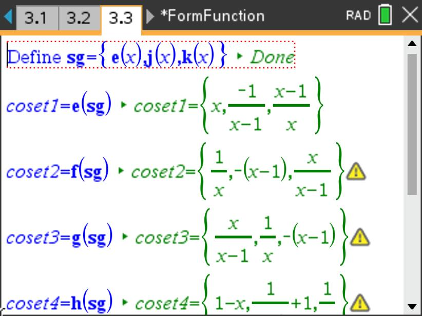
What do you think would happen if we composed a function not found in a specific subgroup with each element in that subgroup? To investigate this question, pick one of the subgroups generated in a column from part (k) and compose it with a function not in the subgroup. For example, using the subgroup \(\langle k \rangle=kord=\left\{e,j,k\right\}\) and composing the elements with, say \(f\text{,}\) we get the new set as shown below. This subset formed by composing \(f\) with \(\langle k \rangle\) is denoted \(f \circ \langle k \rangle\) and called a coset. This can be done in either the Calculator page or the dynamic Notes page as shown below. Note that for your convenience, the Notes page (3.3) allows you to edit the subgroup at the top of the page and all cosets below it are automatically updated. If you prefer, you can use the imbedded GeoGebra applet provided in Figure 4.3.8.
Figure4.3.8.Coset Compositions
(n)
How many elements are in our new coset, \(f \circ \langle k \rangle\text{?}\) Does the new coset form a subgroup? Use the Notes page (3.3) or the GeoGebra applet for composing the elements of \(\langle k \rangle=kord=\left\{e,j,k\right\}\) with the other elements from \(T\) not in \(\langle k \rangle\text{.}\) What do you notice? Describe what you observe if the other element is already in \(\langle k \rangle\) (e.g. compose \(\langle k \rangle\) with all elements from \(\left\{e,j,k\right\}\text{.}\) Explain why your observations would be true.
Definition4.3.9.Coset.
Let \(H\) be a subgroup of a group \(G\text{.}\) Let \(a\) be any fixed element of \(G\text{.}\) Then the set of all products of the form \(ah\) where \(h \in H\) is called a left coset for \(a\) of \(H\) in \(G\) and is denoted by \(aH\text{.}\) Similarly, \(Ha\) is called a right coset of \(H\) in \(G\text{.}\)
(o)
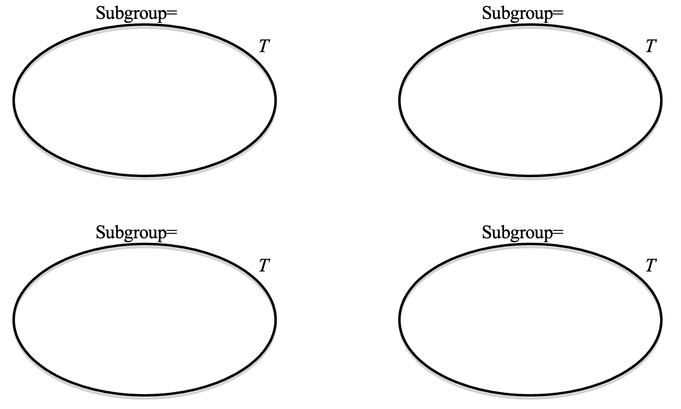
Consider the following diagram of the set, \(T\text{.}\) Draw a boundary around the cosets you found in part (n). An example of the boundary for the coset of the function \(f\) composed with the subgroup \(\left\{e,j,k\right\}\) is shown below. Describe what you notice about the coset boundaries you draw for each situation you found in part (n). Sketch a boundary around the resulting elements in \(T\) below.
(p)
Now repeat what you did in parts (m) & (n) using each different subgroup you found in part (k), sketching boundaries around the cosets formed in the composition of all of the elements from \(T\) with the subgroup. What can you say about the relationship among the cosets formed in each case?
(q)
Do all of the different cosets you found in part (p) form subgroups? If not, under what conditions do they form subgroups?
(r)
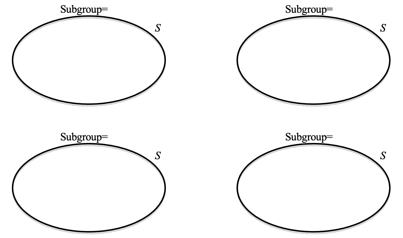
At this point our observations about the partitioning of a group into subsets is based solely on one example of a group. To test your conjectures, first confirm that the following set, \(S\text{,}\) of matrices forms a group under the operation of regular matrix multiplication. To do this, first insert a new problem by pressing doc and selecting \(\mathbf{Insert}\) and then \(\mathbf{Problem}\text{.}\) After selecting a Calculator page, use the Define command to store each matrix by name in memory so that product of, say \(a\) and \(b\text{,}\) can be entered simply as \(a\cdot b\) on the CAS. Now create subgroups of the set by raising each element to increasing powers until you reach the identity, then repeat the process from parts (o) and (p) to see if the group of matrices is partitioned in a similar manner as was the set \(T\) by sketching and circling subsets.
Using the evidence from your diagrams, give an argument for why the order of an element must divide the order of the group. Given that your argument is based on only a few cases of evidence (namely the sets \(T\) and \(S\) with various subgroups), what main properties would you need to show in order to prove your claim in general?
So what are the takeaways from this investigation, specifically for this particular set and operation, as well as for general structures that have the properties of groups? Well, let’s consider the observations you hopefully noticed in the exploration. We can summarize four main ideas here.
From part (k), the order (or size) of the subgroups were either 1, 2, or 3.
From part (n), all cosets were the same size as the subroup that generated the coset.
From part (p), cosets generated by a given subgroup are either completely identical or completely disjoint.
From part (p), all elements of the group occur in exactly one coset, disregarding repeated cosets (i.e. no stragglers lurking outside a coset).
The result of these observations is that the group gets chopped up into disjoint subsets (cosets) all having the same number of elements in them. Since the cosets all have the same size as the subgroup used to generate them, this means that the size (or order) of the subgroup must divide the order of the original group. Hence since our group of functions had order 6, we should only expect a subgroup to have an order that is a divisor of 6. Again, as you noticed in part (k), the sizes of the subgroups were 1, 2, or 3 (all divisors of 6). We can’t have a subgroup of, say order 5, if our group is of order 6 since 5 does not divide 6.
We have observed these patterns in the activity Activity 4.3.6, but will this hold for all groups? In order to be certain, we need to prove it for all groups based on the basic properties of groups. Let’s start by trying to argue these observations a little at a time.
One of the key parts of the argument deals with having all cosets being of the same "size" (actually the size of the subgroup that generated the coset). To establish that this was not just a fluke in our activity, we need to consider what would happen if cosets were not the same size as the subgroup that gave birth to them.
Theorem4.3.10.Coset "Size".
A left (or right) coset in a finite group contains the same number of elements as the subgroup that generated the coset.
Proof.
Suppose \(H \lt G\) (i.e. \(H\) is a subgroup of \(G\)). Further, let \(H=\left\{h_1, h_2, h_3, \ldots, h_m\right\}\text{.}\) Now we can form a left coset, \(aH\text{,}\) such that \(aH=\left\{ah_1, ah_2, ah_3, \ldots, ah_m\right\}\text{.}\) We can claim that all elements of this coset are unique since if not, we must have that \(ah_i=ah_j\text{,}\) for some \(i\) and \(j\) with \(i \neq j\text{.}\) But this would mean that \(a^{-1}ah_i=a^{-1}ah_j \Rightarrow\)\(eh_i=eh_j\text{,}\) and thus \(h_i=h_j\) and so \(ah_i \neq ah_j\text{.}\)
The next observation that we made in Activity 4.3.6 was that if we put all of the cosets together, we ended up with the entire group (as evidenced in your diagrams of cosets).
Theorem4.3.11.Union of Cosets is the Group.
Let \(H\) be a subgroup of a group \(G\text{.}\) Then the union of all left cosets of \(H\) gives the entire group \(G\text{.}\) In other words, \(G=\bigcup\limits_{a \in G}aH\text{.}\)
Proof.
Since every left coset consists of elements from \(G\text{,}\) then \(ah \in G\) for all \(a \in G\) and \(h \in H\text{.}\) Therefore, we have \(\bigcup\limits_{a \in G}aH \subseteq G\text{.}\) Now, if \(b \in G\) and since \(e \in H\text{,}\) we can see that every element of \(G\) can be found in its respective coset, \(bH\text{,}\) since \(b=be \in bH\text{.}\) Since \(b \in G\text{,}\) then \(bH \subseteq \bigcup\limits_{a \in G}aH\) and thus, every element in \(G\) is also in \(\bigcup\limits_{a \in G}aH\text{.}\) Therefore, \(G \subseteq \bigcup\limits_{a \in G}aH\text{.}\) Since \(\bigcup\limits_{a \in G}aH \subseteq G\) and \(G \subseteq \bigcup\limits_{a \in G}aH\text{,}\) we have that \(G=\bigcup\limits_{a \in G}aH\text{.}\) Note that this proof also works for right cosets.
The significance of this theorem is that a group can be formed by the union of all of its left (or right) cosets. But, could some of these cosets overlap in some way? If so, how can the elements from one coset overlap with another? Are there any restrictions on the overlap? You will recall experiencing this partitioning in Activity 4.3.6 lab when you placed boundaries around the subsets from \(T\) that you found as a result of composing subgroups with elements from the set \(T\text{.}\) You will also recall from the activity that the subsets (cosets) did not appear to overlap once you placed the boundaries around them. Put another way, the subsets generated in the activity either had no elements in common or were identical. While our experiences have suggested that there is no overlap, we do need to address this issue of possible overlap from a more formal and absolute sense. Consider the following theorem.
Theorem4.3.12.Coset Overlap.
Let \(H\) be a subgroup of a group \(G\) and let \(a,b \in G\text{.}\) Then we have that any two left cosets \(aH\) and \(bH\) either have no elements in common or are identical.
Proof.
Suppose \(c \in aH\) and \(c \in bH\text{.}\) This means that \(c=ah_1=bh_2\) for some \(h_1, h_2 \in H\text{.}\) Then we must also have that \(a=bh_2h^{-1}_1\text{.}\) This implies that for any \(h_3 \in H\text{,}\) we can express \(ah_3=\left(bh_2h^{-1}_1\right)h_3=b\left(h_2h^{-1}_1b_3\right)=bh_4\) for some \(h_4 \in H\) since \(H\) is closed. From this we can say that \(ah_3=bh_4 \in bH\) and thus every element in \(aH\) is also in \(bH\) implying \(aH \subseteq bH\text{.}\) By a similar argument, we also get that \(bH \subseteq aH\text{,}\) thus \(aH=bH\text{.}\)
We now have everything we need to address the observation that you made from Activity 4.3.6. Recall that when you examined the “powers” of the function composition in the activity, there was an interesting observation made, namely, the orders of the elements (functions in this case) seemed to be a divisor of the order of the group. This brings us to a classic theorem known as LaGrange’s theorem.
Theorem4.3.13.LaGrange’s Theorem.
Let \(G\) be a finite group or order, \(\left| G \right|=n\text{.}\) If \(H \lt G\) (i.e. \(H\) is a subgroup of \(G\)), and \(\left| H \right|=m\text{,}\) then \(m \mid n\text{.}\)
Proof.
Let \(G\) be a finite group and \(H \lt G\) with \(\left| G \right|=n\) and \(\left| H \right|=m\text{.}\) Since \(G\) is finite and each left coset of \(H\) has \(m\) elements by Theorem 4.3.10 with either left cosets being identical or disjoint as shown by Theorem 4.3.12, there must be a finite number, call it \(t\text{,}\) of distinct left cosets of \(H\text{.}\) Since every \(a \in G\) is guaranteed to be in the left coset \(aH\) and together the union of all left cosets gives \(G\) as seen from Theorem 4.3.11, this implies that \(n=mt\) and thus \(m \mid n\text{.}\)
Now that we have spent some time exploring basic properties in algebra through Activity 4.3.6, we can start to examine how these structures relate to the secondary curriculum and how we can engage students in doing more than mimicking symbol manipulation without an understanding of the meaning behind the manipulation. As you discovered earlier, the most basic of structure in algebra is the group since the properties of a group are the minimal needed for use in solving an equation that uses only one operation. Let’s now dig a little deeper into these ideas.
In order to address the underlying structure of mathematics, we will examine a basic skill that is taught in the secondary schools from an advanced standpoint. At this point, it is assumed that the reader has experienced the corresponding parts of this text including the activity Activity 4.3.6 as well as the portions of the Interactive Mathematics Program (IMP) titled, Functions in Verse, Linear Functions in Verse, An Inventory of Inverses, and the Supplemental Problem, Its Own Inverse. In addition, it is also assumed that the reader has discussed the vignette, Inverse Functions: The Case of Tim (Activity 4.3.5). These activities and curriculum materials are essential to give the reader a point of reference for this mathematical discussion on algebraic structure.
Before we begin an examination of algebraic structure and its relationship to the secondary curriculum, we first need to think about the basic components that make up different types of algebraic structures. Generally, when we think about algebra, be it at the secondary or undergraduate level, we have two basic components—a set and an operation or operations.
You may recall from your high school experience a great deal of time spent simplifying or solving expressions or equations that involved primarily the operations of addition, subtraction, multiplication, and division. In these cases, the operations were binary meaning that they took two elements in a set (say the real numbers) and returned another element from the same set. While the result of a binary operation does not have to be from the same set as the inputs, we will restrict our discussion to this case since it is the most familiar. For example, \(2+3=5\) takes the two numbers 2 and 3 and returns the number 5. Similarly with multiplication, \(2 \cdot 3=6\) takes the two numbers 2 and 3 and returns the number 6.
Although arithmetic operations are the basis of many people’s experience within the school setting, we can also think about non-arithmetic operations. Recall from your experiences in the activity, Form and Function, we used the operation of function composition. If you have ever worked a puzzle called Rubik’s Cube, you have performed other non-arithmetic operations. In this case you can describe clockwise rotations of various faces as well as a myriad of other moves that transform the cube from one state to another. As we will see, whether we use arithmetic operations or non-arithmetic ones, there is an underlying structure that becomes evident as we notice patterns of behavior for elements of the set with which the operations are associated.
When we examine the solutions to basic equations, we notice a similar structure that occurs in all processes regardless of the binary operation being used. If we consider the solution to the equation \(a*x=b\) for any binary operation, \(*\text{,}\) the process used to find the solution is the same no matter what operation we choose. However, in order to use this process, there are some underlying assumptions that need to be stated.
Recall in Activity 4.3.1 and Activity 4.3.2 we determined the minimal properties needed to be able to solve an equation in one operation. These properties were what we used to define the most basic of algebraic structures, a group (see Definition 4.3.1). If we examined the steps used in the solution of each of these equations, we will noticed that the statements of properties and definitions as well as the order in which they were applied were identical. In fact, when I was writing these portions of the text, I simply copied and pasted the first solution into the document and then replaced all of the "\(+\) operations with “\(\cdot\)" and then all of the instances of "\(-a\)" were replaced with "\(\frac{1}{a}\)". When we think about writing this section of the text in this way, the algebraic structure becomes very clear.
In order to study algebraic structure, we need to first consider the basic components that make up that structure. As we stated before, generally we think of sets and operations as the building blocks of an algebraic system. Young children become familiar with the concept of set from a very early age through the use of physical manipulatives, but what about operations? How do children view operations? One might argue that many children see arithmetic operations as physical actions that operate on sets of objects. After all, early development of the addition concept involves combining sets of objects.
Others might argue that many children see operations as a series of procedures to be performed using pencil and paper. Traditionally, in elementary school, a great deal of time is devoted to memorizing “addition facts” and “multiplication tables”. Of course, from a traditional point of view, knowing addition and multiplication facts is essential for mastery of the algorithms that follow. One goal of our existing curriculum is to enable students to compute sums and products efficiently and accurately. However, after observing children working on problems within a context, we have begun to question whether or not they make the connection between the earlier physical operations on sets and the arithmetic operations on numbers. In many cases, a child will be able to perform computations such as \(427 \div 3\) while at the same time struggle with a problem like:
Sue, Jan, and Amanda put equal amounts of money together and bought a large tub of candy containing 427 pieces. If they agree to split the candy equally, how many pieces does each get? Are there any pieces left over?
In many instances, the child is able to do the computation when posed simply as, \(427 \div 3=\text{,}\) but does not necessarily have a conceptual understanding of what the quotient, remainder, or divisor represent. This disconnect between conceptual meaning and algorithmic procedure is concerning since in order to apply mathematical processes to real-world problems, the student must first understand what the process means so that it will be applied in an appropriate situation.
For example, in my early years of teaching, I has an experience teaching algebraic concepts related to distance, rate, and time. I asked a student the question, “If you drive at 55 mph for two hours, how far have you traveled?” Upon first consideration, the student simply looked puzzled. In response, thinking the student was having trouble doubling 55, I changed the problem by saying, “Suppose you drive at 60 mph for two hours, how far have you traveled?” \(-\) I thought doubling 6 might be easier. The student replied, “Three miles.” What was the student doing? Upon further probing, it turns out that the student was simply dividing 60 by 2 (incorrectly) because he had been taught that you “divide when you have distance, rate, and time problems.” It comes as little surprise that this same student when posed with a new problem and asked how he might solve it responded, “Add…, no subtract…, no divide.” After uttering each response, he would watch my face looking for cues as to which operation was correct. I referred to this student approach as the “random operator generator”. It is important to note that this student was fairly proficient at computing with pencil and paper algorithms. The bottom line is that this student had very weak (if not nonexistent) connections between algorithmic procedures and conceptual understanding of the operations in question. If unable to make conceptual connections, there is very little chance that the student will be able to solve mathematical problems. So what good is computational proficiency, if the student does not know when it is appropriate to employ a certain type of computation?
Functions, Mappings, and Binary Operations
As we think about teaching children operations and the algebraic properties that are associated with them, it is helpful to put ourselves in the same unfamiliar position as our students by considering operations that are not familiar to us. But how do we create operations other than addition, subtraction, multiplication, and division? We could use operations from linear algebra where properties such as commutativity are no longer assumed. However, we can also create our own operations that are combinations of familiar ones. Once created, we can then investigate properties and even attempt to solve equations that use the operation.
Suppose we want to explore a binary operation, call it \(*\text{,}\) on the set of real numbers defined by \(a*b=a+b-a\cdot b\) where "\(+\)" and "\(\cdot\)" are the familiar operations of addition and multiplication. It would be nice if we could define this operation and then explore it using technology. In order to do this, let’s first consider viewing a binary operation in a different way. As we discussed earlier, a binary operation takes two inputs, in this case from the set of real numbers, and yields a result that it also a real number. In algebra, we have seen another construct that also behaves in this manner (especially if we thinking back to Calculus 3). In a sense, a function takes inputs and produces outputs associated by the function rule. In this situation we want two inputs to yield a single output and so we can use a function of two variables. Here we can let a function, call it \(\varphi\text{,}\) be defined such that \(\varphi : \mathbb{R} \times \mathbb{R} \rightarrow \mathbb{R}\) and \(\varphi : \left(a,b\right) \mapsto a+b-a\cdot b\text{.}\) In this case, \(\varphi \left(a,b\right)\) acts like the binary operation \(a*b\text{.}\) The advantage of using a function approach to representing a binary operation is that we can use it to define the operation on a computer algebra system (CAS) and then explore the properties of “\(*\)” via the symbol manipulation capabilities of the CAS.
Activity4.3.7.Using Binary Operations.
In this activity, we will explore a binary operation for which we have little intuition. This will allow us to focus on the meaning of algebraic properties more deeply since we cannot use our "common knowledge" to skip over how objects in a set (like the real numbers or integers) behave because we are too familiar with their behavior.
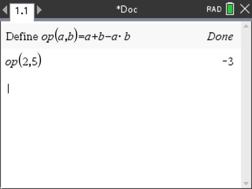
To begin, we are going to define the binary operation, \(*\text{,}\) that was describe above on our CAS so that we can manipulate expressions more easily. To do this, let’s define the operation by using a function of two variables calling it \(op\left(a,b\right)=a+b-a \cdot b\) as shown below.
(a)
Using your defined operation, \(*\text{,}\) on your CAS, explain whether or not it meets the first property of a group, closure. You may want to try to compute several cases like the one shown above for \(2*5=-3\) to convince yourself one way or the other. Can you think of a case where it would not be closed for the integers? For the real numbers? Explain your reasoning.
(b)
Assuming we are using the real numbers, \(\mathbb{R}\text{,}\) as our set, compute several cases like \(2*\left(3*5\right)\) and \(\left(2*3\right)*5\) to give some evidence of whether or not the operation, \(*\text{,}\) is associative. If it is, provide an argument to show it will be for any \(a,b,c \in \mathbb{R}\text{.}\)
(c)
Determine if \(\mathbb{R}\) has an identity element for \(*\text{.}\) If it does, what is it?
(d)
Determine if all elements of \(\mathbb{R}\) have an inverse under the operation \(*\text{.}\) If so, does \(\left(\mathbb{R}, * \right)\) form a group? If not, can you slightly adjust the set \(\mathbb{R}\) so that it does form a group? Explain your reasoning.
(e)
Think back to basic operations like multiplication or addition with real numbers. Have you seen any type of operation that needs a slight adjustment in order to form a group? How does is the behavior from part (d) similar? How is it different?
Since algebra gives us a way to look for regularity and structure, it is particularly useful for reasoning about mathematical ideas. Unfortunately, much of the traditional curricula has focused on primarily procedural knowledge and less on conceptual connections that are present in the procedural processes we spend so much of our time trying to perfect in our students. Gray & Tall (1994) coined the term procept to describe the duality of both the processes in mathematics and the concepts that those processes represent. For this reason, we cannot simple focus on one without the other. Our traditional curricula have often favored the processes and neglected the concepts that those processes use. Since technology has enabled much of the procedural skills to be off-loaded to machines that can perform these procedures more quickly and with far fewer errors, we can de-emphize (not eliminate) the need for procedural fluency so that time can be focused more toward the understanding of the concepts and procedures as part of the same procept. For this reason, let’s consider a situation where a teacher has chosen a task for classroom exploration and try to gain insight into her decision to include this task.
Activity4.3.8.What’s It All About?
Sarah is teaching an algebra class and is trying to get her students to understand some of the underlying structure of algebra. She poses the following question for her students.
"In your groups I want you to consider the following equation, \(\left(x^2-5x+5\right)^{x^2-9x+20}=1\text{.}\) Without using any technology (at least yet), discuss how you might approach solving this equation."
(a)
In your groups, discuss the task and identify the major and minor mathematical concepts involved in solving the equation. List these concepts in order of your perceived importance on your whiteboards under headings of "Major" and "Minor" with "1" being the highest priority concept you think Sarah is trying to address.
(b)
Discuss in your groups why you think Sarah chose this this particular task. What are some features of the equation that are particularly helpful for Sarah’s purpose?
(c)
Now in your groups, carry out a solution of the task without the use of technology. Summarize your solution on your whiteboards and be prepared to share your approach.
(d)
Making use of techology, find a solution of the task. How was your approach different? How was it similar? Did you find the same solutions as when you did not use technology? Explain.
(e)
Reflecting on your original responses to part (a), does your act of solving the problem change your views of what the major and minor concepts of the task are? Explain.
Exercises4.3.4Exercises
1.
Using your CAS and defining \(a*b=a+b-a \cdot b\text{,}\) find the solution(s) to the following equations. Be certain to state your CAS-defined operations and the commands you used to find the solution.
(a)
\(3*x=-9\)
(b)
\(\left(7*x\right)*y=-35\) and \(3*x=-11*y\)
2.
Consider the operation \(*\) given by \(a*b=a+b-5\text{.}\) Verify or refute the following properties. Assume the set under this operation is the set of real numbers. You may need to decide to restrict the set based on what you discover regarding the operation and its relationship to the properties (and a desire for it to be a group). If so, please explain your reasoning for the restriction.
(a)
Closure
(b)
Associativity
(c)
Identity
(d)
Inverses
(e)
Commutativity
3.
Consider the operation \(*\) given by \(a*b=\text{max} \left(a,b\right)\text{.}\) Verify or refute the following properties. Assume the set under this operation is the set of real numbers. You may need to decide to restrict the set based on what you discover regarding the operation and its relationship to the properties. If so, please explain your reasoning for the restriction.
(a)
Closure
(b)
Associativity
(c)
Identity
(d)
Inverses
(e)
Commutativity
4.
Use your CAS to show that \(G=\left\{
\begin{bmatrix}
a \amp b\\
-b \amp a
\end{bmatrix} \mid a,b \in \mathbb{R} \text{ and not both zero} \right\}\) is a group under matrix multiplication. Further, show that \(G\) also has the property of commutativity. A group that is also commutative is called abelian.
5.
Show that the set of 8 symmetries of a square (four rotations and 4 flips) is a group.
6.
Consider \(SL\left(2, \mathbb{R}\right)\) which is defined to be the set of all \(2 \times 2\) matrices of the form \(\begin{bmatrix}
a \amp b\\
c \amp d
\end{bmatrix}\) such that \(a,b,c,d \in \mathbb{R}\) and \(ad-bc=1\text{.}\) Show that \(SL\left(2, \mathbb{R}\right)\) is a group under matrix multiplication. This is called the special linear group—hence the “SL” in the notation.
7.
Suppose that \(G\) is a group and \(a,b,c \in G\text{.}\) Show that if \(ab=ac\text{,}\) then \(b=c\text{.}\)
8.
Suppose that \(G\) is a cyclic group. Explain why it must therefore be abelian. Note that if a group is cyclic, there must be at least one generator (i.e. an element for which all elements in \(G\) can be expressed as a power of it).
9.
Create a set of 8 complex numbers that form a cyclic group under multiplication and identify all elements of the group that are generators.
(a)
List all elements and their inverses.
(b)
Find the orders of each element of the group and describe any patterns you notice with respect to their inverse’s order.
10.
Let \(G=\left\{
\begin{bmatrix}
a \amp a\\
a \amp a
\end{bmatrix} \mid a \in \mathbb{R}, a \neq 0 \right \}
\text{.}\) Show that \(G\) is a group under matrix multiplication. Explain why each element of \(G\) has an inverse even though the matrices have determinants of 0.
11.
Consider the following activity from the High School curricula, Interactive Mathematics Program (IMP), 4th year text, Its Own Inverse (IMP, 2000, p. 155).
In Linear Functions In Verse, \(f\) was an arbitrary linear function defined by the equation \(f\left(x\right)=ax+b\) (with \(a \neq 0\)). You needed to find an expression for \(f^{-1}\left(x\right)\text{.}\) Which linear functions are their own inverses? That is, for what choices of \(a\) and \(b\) is \(f\) equal to \(f^{-1}\text{?}\) (Note: There are infinitely many possibilities.)
12.
Consider the invertible function, \(f\left(x\right)=x^3+2\text{.}\)
(a)
In words, describe what you would do with an input for \(f\) to evaluate it at that value.
(b)
Using your words from part (a) and the process of "undoing", give an expression for \(f^{-1}\text{.}\)
(c)
Graph both \(f\) and \(f^{-1}\) on the same axes. Describe any symmetry you see with these graphs.
(d)
How can the graphical relationship you see in part (c) help with answering exercise 11? Does it support your responses to exercise 11? Explain.
(e)
Examining your experiences in Activity 4.3.6, does this graphical observation support what you found for elements of order 2? Explain.